Curve fitting

Introdução

It may be beneficial to approximate a succession of data points to mathematical functions. Technically,
the described operation is generally called curve fitting/regression. The main applications of curve
fitting are the following:

To summarize, and visualize relationships between input (features/independent variable) and output (target/dependent variable)
To infer function values in intervals where no data is available
To transmit information without passing all the values of the data points
To obtain integrals and derivatives by analytical rather than numerical methods

Given a family of functions that best fits the data points, the problem boils down to obtaining the
best values of the function parameters. The method used depends on the function type. When this
information is not known, it is common to start by plotting the data and try to fit it with various
families of functions.

Taken the example of the data represented in the graph below, it will be described multiple methods to fit to a proper function.

Example data to be fitted by a proper function

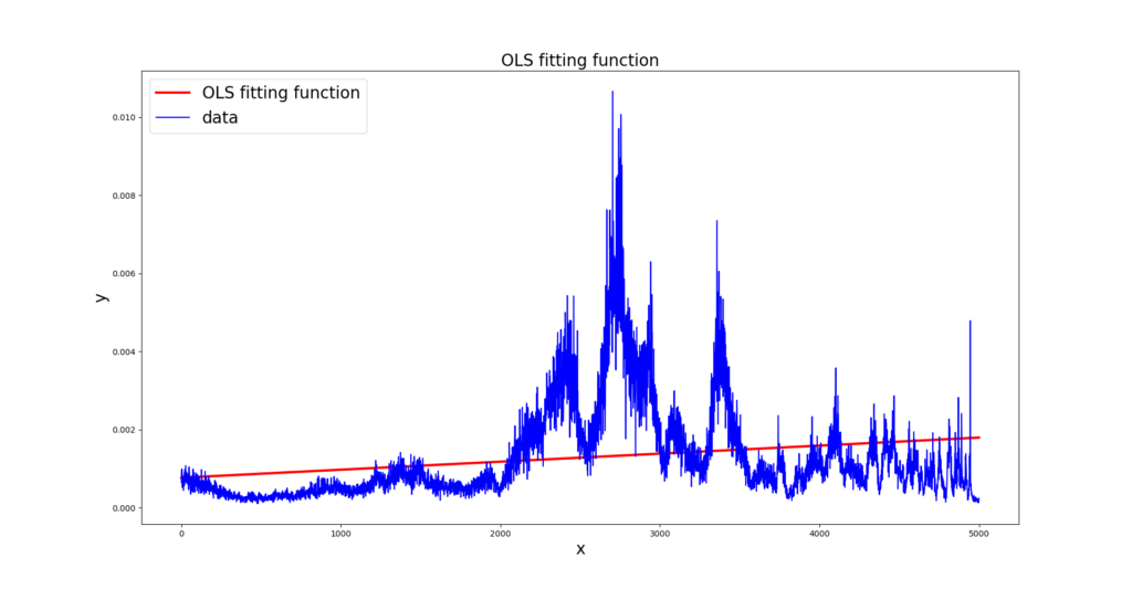
Ordinary least square

Linear regression is one of the simplest algorithms to fit data, using a linear function to describe the
relationship between input and the target variable. It’s clearly inadequate to model our data, but it
will be presented here shortly, for information purpose.

The most common techniques for estimating the parameters in linear regression are based on
minimizing the vertical distance between the estimated plane and the measurements. Among these
techniques, the most popular is Ordinary Least Squares (OLS). The algorithm takes the assumption
that the parameters have equal variance and are uncorrelated. Also assumes the noise to be white and
follows a Gaussian distribution (homoscedasticity).

OLS equation for univariate (having only one variable/input $x$ and a target $y$ ) linear regression can
be written as:

$\boldsymbol{\hat{y}} =\beta\boldsymbol{x}$

We want to minimize $E(\beta)$ which is the sum of squares of the deviations in $\hat{y}$ , from each $y$ -value. In other words, the goal of OLS is to minimize the difference between the real $y$ and the estimate $\hat{y}$ as follows:

(1) $\begin{equation*} E(\beta) = \sum_{i=1}^m [ \hat{y}(x_i) - y_i ]^2 \end{equation*}$

$\beta$ is obtained as by:

(2) $\begin{equation*} \beta=\boldsymbol{(X'X)^{-1}(X'y)} \end{equation*}$

where $\boldsymbol{X}$ is the matrix with the feature values, and $\boldsymbol{X'}$ is its transverse.

The result of the application of OLS to our example is presented in next Figure.

Linear regression of example data by OLS.

Polynomial Least square

In order to fit data with functions which are nonlinear, such as polynomials, least-squares fitting can also be utilized. This technique must find the coefficients $\boldsymbol{a}$ of a polynomial function, of degree $n$ , that best fits the data. Let ( $x_1,y_1$ ),( $x_2,y_2$ ),. . .,( $x_m,y_m$ ) be the data points that need to be approximated by a polynomial function. The least-squares polynomial have the form:

(3) $\begin{equation*} p_n(x) = \sum_{j=0}^n a_jx^j \end{equation*}$

As in the linear case, the coefficients $\boldsymbol{a}$ can be obtained by:

(4) $\begin{equation*} \boldsymbol{a}=\boldsymbol{(A'A)^{-1}(A'y)} \end{equation*}$

where:

$\boldsymbol{A}$ = $\begin{bmatrix} 1 & x_0 & x_0 ^2& . & . & . &x_0^n \\ 1 & x_1 & x_1 ^2 & . & . & . &x_1^n \\ 1 & x_2 & x_2 ^2& . & . & . & x_2^n \\ . & . & . &. & & & . \\ . & . & . & &. & & .\\ . & . & . & & &. & .\\ 1 & x_m & x_m^2 & . & . & . & x_m^n \end{bmatrix}$ , $\boldsymbol{a}$ = $\begin{bmatrix} a_0\\a_1\\a_2\\.\\.\\.\\a_n \end{bmatrix}$ , $\boldsymbol{y}$ = $\begin{bmatrix} y_1\\y_2\\y3\\.\\.\\.\\y_n \end{bmatrix}$

This equations can be used to compute the coefficients of any linear combination of functions $\phi_j(x)_{j=0}^{n}$ that best fits data, since that these functions are linearly independent. In this general case, the entries of the matrix $A$ are given by $a_{ij}=\phi_i(x_j)$ , for $i$ = 1,2,…,m and $j$ = 0,1,…,n.

In the Figure below is represented the approximation of our example to a polynomial function of degree $n=10$ .

Polynomial approximation of example data by Least Squares.

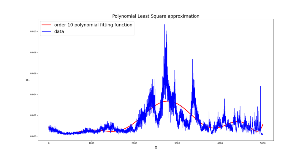
We notice that, even with a high degree ( $n=10$ ), the polynomial doesn’t fit properly to our data, being not able to fit the main data peaks. This is due to the large variation on data behaviour through the dominium of $x$ . Increasing or decreasing polynomial degree doesn’t lead to any better result. In addition, for larger orders of $n$ Runge’s phenomena starts to appear, leading to oscillations on the edges of the interval of $x$ .

Gaussian Approximation with Levenberg-Marquardt

Levenberg Marquardt is a different method to solve the minimization problem in non-linear least squares curve fitting problems. It is used to obtain the parameters $\boldsymbol{\beta}$ of any function $f(x_i,\boldsymbol{\beta})$ we want to approximate the data to. Levenberg Marquardt algorithm (LM) is a iterative procedure that converges fast, but it finds only local minimum, instead of global minimum. So it deeply depends on the initial guess of the parameters.

The objective of this algorithm is to obtain $\boldsymbol{\beta}$ values by minimizing $S(\boldsymbol{\beta})$ :

(5) $\begin{equation*} S(\boldsymbol{\beta}) = \sum_{i=1}^m [y_i - f(x_i,\boldsymbol{\beta})]^2 \end{equation*}$

In each iteration step, the parameter vector $\boldsymbol{\beta}$ is replaced by a new estimate $\boldsymbol{\beta} + \delta$ . To determine $\delta$ , the function $f\left(x_{i},\boldsymbol{\beta}+ \delta\right)$ is approximated by its linearization:

$\begin{equation*} f(x_i,\boldsymbol{\beta} +\boldsymbol{\delta}) \approx f(x_i, \boldsymbol{\beta}) + \boldsymbol{J_i} \delta, \end{equation*}$

where

$\begin{equation*} \boldsymbol{J_i}= \frac{\partial f (x_i,\boldsymbol{\beta})}{\partial \boldsymbol{\beta}} \end{equation*}$

Substituting in the equation 5, rearranging and taking the derivative with respect to $\boldsymbol{\delta}$ and setting the result to zero, we have:

$\begin{equation*} \boldsymbol{\delta}=(\boldsymbol{J^TJ} + \lambda \boldsymbol{I})^{-1}(\boldsymbol{J}^T\epsilon) \end{equation*}$

where $\lambda$ is a damping parameter adjusted at each iteration and $\boldsymbol{\epsilon=y}-f(\boldsymbol{\beta})$ .

LM is adaptive because it controls its own damping: it raises the damping parameter if a step fails to reduce the error $\boldsymbol{\epsilon=y}$ ; otherwise it reduces the damping. In this way LM is capable to alternate between a slow descent approach when being far from the minimum and a fast convergence when being at the minimum’s neighborhood. There are several method to update damping parameter $\lambda$ .

To illustrate Levenberg Marquardt application, it was used to approximate our example data points to a set of Gaussian functions. The example is presented in the next Figure.

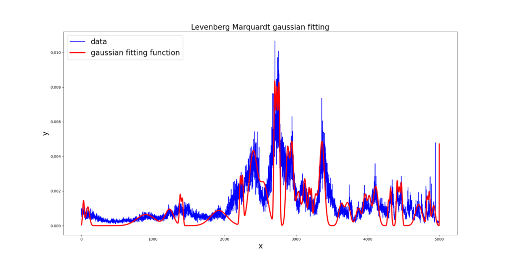
Gaussian approximation of example data by Levenberg-Marquardt

The result was better than polynomial approximation case, as this one captures the main data
peaks. However, the edges of those peaks are not properly adjusted.

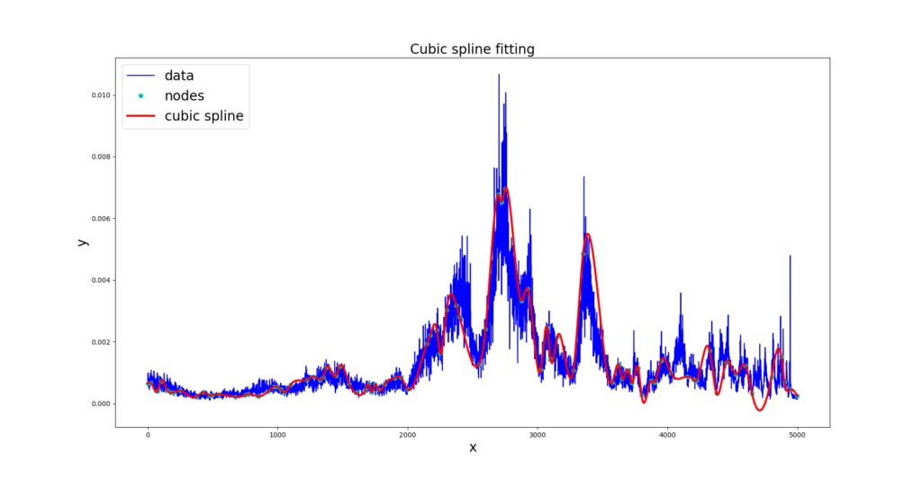
Cubic Spline

Cubic spline approximation is a method to fit data to a cubic piecewise polynomial. For that, the data is divided into several segments and each of those segments is modeled by a cubic polynomial. These segments are delimited by nodes, which are the local maximum or minimum of the data set. Each two consecutive nodes are interpolated by a cubic polynomial. If there are n knots points ( $(x_1,y_1),(x_2,y_2)…(x_n,y_n)$ ), there are n-1 segments each defined by a cubic polynomial $S_i(x)$ , as follow:

$\begin{equation*} S_{n-1}(x)=y_{n-1}+b_{n-1}(x-x_{n-1})+c_{n-1}(x-x_{n-1})^2+d_{n-1}(x-x_{n-1})^3 \text{ } on \text{ } [x_{n-1},x_n] \end{equation*}$

The coefficients for each polynomial are obtained solving the following system of equations that guarantees the continuity and smoothness of the final total spline function.

(6) $\begin{equation*} S_i(x_i)=y_i \text{ } \text{ and } S_i(x_{i+1})=y_{i+1} \text{ } for \text{ } i=1,2,...,n-1 \end{equation*}$

(7) $\begin{equation*} S'_{i-1}(x_i)= S'_{i}(x_i) \text{ } for \text{ } i=1,2,...,n-1 \end{equation*}$

(8) $\begin{equation*} S''_{i-1}(x_i)= S''_{i}(x_i) \text{ } for \text{ } i=1,2,...,n-1 \end{equation*}$

In our example, the system of equations was solved using iterative Jacobi method, and the result is in next Figure.

Cubic spline approximation of example data.

Conclusion

In this article, the main methods of curve fitting data were discussed. Variations of the methods
presented are often used, and other alternatives are available. Methods based on gradient descent are
an alternative in solving linear and nonlinear regression problems.

Referências

[Hay02] Simon S Haykin. Adaptive filter theory. Pearson Education India, 2002.
[Lou05] Manolis Lourakis. A brief description of the levenberg-marquardt algorithm implemened by levmar. A Brief Description of the Levenberg-Marquardt Algorithm Implemented by Levmar, 4, 01 2005.
[Win] Natural cubic splines implementation with python. https://medium.com/eatpredlove/natural-cubic-splines-implementation-with-python-edf68feb57aa. Accessed: 2022-12-05.

Autor

Bárbara Matos

Blog

Introdução

Ordinary least square

Polynomial Least square

Gaussian Approximation with Levenberg-Marquardt

Cubic Spline

Conclusion

Referências

Autor

Equipment Revamping

First-Principle Modelling

Deixa aqui o que pensas sobre este artigo: Cancelar resposta

Artigos recentes

Comentários recentes